
Accuracy and Validation 2025
1. Executive Summary
TomTom Historical Traffic Volumes estimates how much traffic uses each road segment in the network, at both daily and hourly resolution, using machine learning applied to probe data from millions of connected devices worldwide. It reports annual average daily traffic (AADT), average annual weekday hourly traffic (AAWHT) — the typical volume for each hour of a weekday — and estimates for individual hours of the day. Unlike traditional counting methods that require physical equipment at each measurement point, this approach generates estimates for any road segment where TomTom map and probe data are available.
The hour-by-hour estimates cover historical periods from 2024 onward and are kept current to within approximately 72 hours of the present.
A rigorous accuracy assessment was conducted using independent ground-truth traffic counts from permanent loop detectors and similar counting infrastructure across seven countries — Belgium, United Kingdom, Netherlands, Norway, New Zealand, Sweden, and United States — for 2025. All validation metrics are derived from k-fold cross-validation, which tests the model against data it was not trained on, giving a reliable indication of real-world performance. Section 6 describes the complementary Leave-One-Country-Out (LOCO) validation approach used for markets beyond these seven countries.
Key findings:
- The United Kingdom is the strongest performer in this assessment, with an all-roads AADT MAPE of 4.0% and a Very Good SQV (0.90 or better) sustained in every volume band; its high-volume band reaches a MAPE of 2.3%.
- Across the seven countries, all-roads AADT MAPE ranges from 4.0% (United Kingdom) to 10.0% (New Zealand); Norway pairs a high MAPE of 9.3% with a Very Good SQV of 0.90, showing that errors remain well-controlled in absolute terms.
- Percentage errors are consistently higher on low-volume roads in every country, but on such roads they correspond to small absolute vehicle counts; Section 8 provides guidance on interpreting these values.
2. Introduction: Why Validation Matters
Traffic volume data is used to make consequential decisions:
- Where to locate a retail outlet
- How to allocate infrastructure budgets
- How to assess road safety risk
- Whether a proposed development can be supported by the surrounding road network
For these decisions to be sound, the underlying data must be reliable. For customers to make that judgment, they need to understand, in practical terms, how accurate the data actually is.
Traditional counting methods provide precise counts at a small number of fixed points. TomTom Historical Traffic Volumes, however, generates estimates for every road segment in the network. Because estimation involves uncertainty, our approach transparently quantifies that uncertainty using accepted industry metrics, enabling customers to make an informed decision about where and how to use the data.
Validation is conducted using data from permanent counting stations — independent ground-truth counts that were not used in model training. The accuracy metrics in this paper measure the gap between TomTom estimates and those independent reference counts. A smaller gap means a more accurate estimate. Where results fall short of quality thresholds, this paper says so clearly, with available context.
3. How the Model Works
TomTom Historical Traffic Volumes is produced by a three-stage pipeline. Each stage addresses a distinct challenge in translating raw observations from connected vehicles into reliable, network-wide volume estimates.
3.1 From connected vehicles to traffic observations
The primary data source is floating-car data (FCD): GPS and telematics signals from connected vehicles. Connected vehicles include:
- In-vehicle navigation systems
- Smartphones running navigation apps
- Connected commercial vehicles
These signals are collected passively and continuously from millions of devices worldwide. For each road segment, this data provides a continuous stream of speed and passage observations.
Raw probe observations, however, do not equal traffic volumes. Only a fraction of all vehicles traveling on any given road are connected and contributing data. This fraction, the penetration rate, varies by road type, geography, and time of day. Accurately converting probe observations into total volume estimates requires explicitly accounting for this variation.
3.2 Estimating probe data representativeness
A core challenge in probe-based traffic modelling is that the proportion of vehicles captured by probe data differs across roads and regions. A major urban motorway may have high connected-vehicle penetration; a rural minor road may have very low penetration. Without correcting for this, estimates would systematically over-represent well-instrumented road types and under-represent others, producing results that are not comparable across a network.
The model estimates penetration rates continuously across the road network, using traffic-state signals from probe data combined with map attributes such as road class, urban or rural context, and lane configuration. Roads operating at or near capacity provide the most reliable signal for this estimation, because the physical relationship between vehicle speed and traffic flow becomes predictable in congested conditions. These estimates are aggregated and smoothed to produce a spatially consistent representation of probe coverage that supports all volume estimates.
3.3 Predicting total traffic volumes: a Mixture-of-Experts approach
With penetration-rate estimates in hand, the model converts probe observations into absolute vehicle counts using a Mixture-of-Experts (MoE) volume model.
The motivation is straightforward: different types of roads follow different traffic patterns. A motorway and a residential street each have their own relationship between road characteristics and traffic load. A single model that attempts to fit both will inevitably compromise the accuracy of one or both road types. Rather than accepting that trade-off, the MoE model uses two specialized components: one trained primarily on high-volume roads, and another on lower-volume roads. A third component, the gating network, learns from the characteristics of each road segment which blend of the two specialist components is most appropriate. For a road that clearly resembles a busy arterial, the model draws heavily from the high-volume component. For ambiguous cases, it applies a weighted combination, producing smooth and consistent predictions across the full range of road types.
The volume model produces baseline estimates first: annual average daily traffic (AADT) for each segment, and average annual weekday hourly traffic (AAWHT) — the typical volume for each hour of a weekday.
Estimates for individual hours build on these baselines, informed by the traffic observed in each period.
A final calibration step adjusts estimates by road class and region to reduce systematic bias.
4. How We Measure Accuracy
Accuracy is reported using a set of complementary metrics. Each highlights a different aspect of model performance. Together they give a complete picture of how estimates compare to independent ground-truth counts.
| Metric | What it measures |
|---|---|
| MAPE (Mean Absolute Percentage Error) | The average percentage by which estimates differ from actual counts, regardless of direction. The primary summary measure. Lower is better. |
| Median Percentage Error | The middle value of all signed errors. Indicates systematic bias: positive = tendency to over-predict; negative = tendency to under-predict. Values close to zero are ideal. |
| 68th and 95th Percentile APE | The spread of errors across road segments. The 68th percentile covers roughly one standard deviation; the 95th captures the tail of the distribution where the model is most challenged. |
| SQV (Scalable Quality Value, 15th Pct) | A bounded quality score (0 to 1) designed to be consistent across roads of all volumes. Reported at the 15th percentile: at least 85% of segments perform better than this value. |
| MAE (Mean Absolute Error) | The average number of vehicles per hour by which estimates differ from actual counts, regardless of direction. Reported for hourly volumes, it expresses error in real traffic units rather than percentages. Lower is better. |
4.1 Mean Absolute Percentage Error (MAPE)
MAPE measures the average magnitude of prediction errors relative to the observed count, expressed as a percentage. A MAPE of 10% means that, on average, estimates differ from actual counts by 10%. MAPE treats errors of all sizes equally and is the most widely reported accuracy measure in traffic estimation literature.
An important characteristic of MAPE: on very low-volume roads, a high percentage error may represent a small absolute difference in vehicle count. A road with 300 vehicles per day and a MAPE of 15% has a typical absolute error of roughly 45 vehicles. For most planning and analytical purposes, this absolute difference is negligible. Users should interpret MAPE values for low-volume roads alongside the absolute volume context for their use case.
4.2 Median Percentage Error
The Median Percentage Error is the middle value of all signed errors (positive when our estimate exceeds the actual count, negative when it falls short). A value close to zero indicates that the model has no strong tendency to over- or under-count. For applications such as aggregated network analysis or vehicle kilometres travelled (VKT) calculations, low bias is important because systematic errors accumulate across many road segments.
4.3 68th and 95th Percentile Absolute Percentage Error
These percentiles describe the spread of errors across road segments. The 68th percentile is roughly equivalent to one standard deviation in a normal distribution, describing the error level that approximately 68% of segments fall within. The 95th percentile captures the upper range, showing the level of error experienced by the most challenging segments. Together, these metrics give a more complete picture of how error is distributed than MAPE alone.
4.4 Scalable Quality Value (SQV)
The Scalable Quality Value (Friedrich et al., 2019) is a bounded, scale-independent quality metric that produces a score between 0 and 1, where 1 represents a perfect match. It is designed to perform consistently across the full range of traffic volumes. SQV is reported as its 15th percentile across all segments in each group: at least 85% of road segments in the group perform better than the stated value. The quality thresholds below are taken from Friedrich et al. (2019):
| SQV | Assessment | Guidance for use |
|---|---|---|
| ≥ 0.90 | Very good | High confidence in segment-level comparisons. Suitable for precision analytics and granular planning. |
| ≥ 0.85 | Good | Suitable for cross-segment analysis and most planning applications. |
| ≥ 0.80 | Acceptable | Suitable for network-level planning and transport modeling. Validate individual segments where precision matters. |
| Below 0.80 | Below threshold | Use with caution. Treat results as indicative and validate against local count data where possible. |
4.5 Mean Absolute Error (MAE)
MAE measures the average absolute difference between predicted and observed volumes, expressed in vehicles per hour. It is reported for hourly volumes and answers a question the percentage-based metrics cannot: by how many vehicles per hour does a typical estimate differ from the actual count? An MAE of 30 means that, on average, hourly estimates differ from actual counts by 30 vehicles.
MAE complements MAPE (Section 4.1). Because it is measured in the same units as the traffic itself, MAE is not inflated by the small denominators of quiet roads and quiet hours, where a difference of a few vehicles can register as a large percentage error. Conversely, MAE is dominated by high-volume roads, where the same relative error corresponds to many more vehicles. MAE values are therefore most meaningful when compared within a volume category or road class and should be read alongside the percentage-based metrics rather than in isolation.
4.6 R² (Coefficient of Determination)
R² (the coefficient of determination) measures how much of the variation in true traffic volumes is explained by the model’s predictions, on a scale where 1.0 represents a perfect match and 0 indicates the model performs no better than simply predicting the average volume for every segment. Unlike MAPE or SQV, which describe the typical size of an error, R² describes how well the model captures the overall pattern of high- versus low-volume roads across the network.
R² is most useful as a network-level diagnostic: a high R² indicates the model correctly distinguishes busy roads from quiet ones even if individual segment-level errors remain, which is relevant for use cases such as relative ranking of road segments, network-wide planning, or identifying whether the model captures real-world volume variation rather than regressing toward an average. Because R² is sensitive to the range of volumes included in a sample, it is reported here at country level and, where sample sizes allow, by volume category, alongside the other metrics in this section — it should be read together with MAPE and SQV rather than in isolation, since a strong R² does not on its own guarantee small errors on any single segment.
5. Validation Approach: K-Fold Cross-Validation
All accuracy metrics in this paper are derived from k-fold cross-validation. This method tests the model against data it was not trained on, giving a realistic and unbiased measure of real-world performance.
The countries used in the training process are divided into groups (folds). In each iteration, one group is held back entirely; the model is trained on the remaining groups and then evaluated against the held-back group. This process repeats until every group has served as the test set. Accuracy figures are aggregated across all test iterations, so every validation counter contributes to the reported results without ever being used to train the model it is evaluated against.
K-fold cross-validation is standard practice in machine learning validation because it prevents overfitting to the test set, uses all available ground-truth data efficiently, and produces a reliable estimate of generalisation performance.
Validation counters are drawn from permanent loop detectors and similar permanent counting infrastructure. Results are reported for three volume categories:
- High-volume roads: 55,000 or more vehicles per day (AADT)
- Medium-volume roads: 5,000 to 54,999 vehicles per day
- Low-volume roads: fewer than 5,000 vehicles per day
An All roads row in each results table presents aggregated metrics across all counters in the country, regardless of volume category.
K-fold cross-validation requires ground-truth counting data for every country in the validation set. Section 6 describes the complementary Leave-One-Country-Out (LOCO) approach used to estimate accuracy in markets where no counter data exists.
6. Leave-One-Country-Out (LOCO) Validation
TomTom Historical Traffic Volumes is available in many markets where no permanent counting infrastructure exists. K-fold cross-validation, described in Section 5, requires ground-truth data and therefore cannot be applied directly to these markets. Leave-One-Country-Out (LOCO) validation addresses this by providing a principled method for estimating accuracy in unseen markets.
6.1 How LOCO validation works
In LOCO validation, one country is entirely excluded from model training. The model is trained on all remaining countries and then evaluated against the held-out country using the counter data available there. This process repeats for each country in turn, so that every country serves once as an unseen test market.
The key distinction from standard k-fold cross-validation is that LOCO simulates deployment in a market where the model has had no prior exposure to local data. The accuracy results from LOCO validation therefore represent a realistic estimate of performance in new markets — markets where the model must rely entirely on what it has learned from other countries.
6.2 Why LOCO matters for customers
For customers using TomTom Historical Traffic Volumes in markets beyond the seven countries covered in Section 7, LOCO validation results provide the primary quality basis. Because the model learns traffic patterns that generalize across countries — road network structure, speed-flow relationships, penetration rate dynamics — LOCO results typically remain within an acceptable accuracy range even in markets the model has not directly observed.
6.3 LOCO Results Coming Soon
LOCO results will be provided once countries are ready for launch; where LOCO results indicate reduced accuracy for specific road categories in specific markets, this will be documented and made available to customers. This transparency will be an extension of the k-fold results in Section 7 to the full set of markets where the product is available.
7. Results (2025)
The following tables present accuracy results for each of the seven countries in the 2025 k-fold validation. Quality tiers for the SQV (15th Pct) values are defined in Section 4.4.
7.1 Belgium
AADT
| Road Category | Counters | MAPE (%) | 68th Pct APE (%) | 95th Pct APE (%) | Median PE (%) | SQV (15th Pct) |
|---|---|---|---|---|---|---|
| All roads | 1,730 | 7.1 | 8.1 | 20.1 | -0.4 | 0.88 |
| High (55,000+) | 128 | 4.1 | 4.5 | 14.2 | -0.9 | 0.85 |
| Medium (5,000–54,999) | 1,100 | 6.5 | 7.5 | 17.5 | -0.7 | 0.87 |
| Low (under 5,000) | 502 | 9.2 | 11.1 | 24.4 | 0.8 | 0.92 |
Hourly
Day hours (06:00–23:00)
| Road Category | Counters | MAE (veh/h) | MAPE (%) | 68th Pct APE (%) | 95th Pct APE (%) | Median PE (%) | SQV (15th Pct) |
|---|---|---|---|---|---|---|---|
| All roads | 1,622 | 87.1 | 11.8 | 12.3 | 32.2 | -0.5 | 0.88 |
| High (55,000+) | 123 | 220.5 | 7.1 | 7.5 | 17.8 | -1.5 | 0.83 |
| Medium (5,000–54,999) | 1,025 | 94.1 | 10.6 | 11.1 | 27.2 | -0.5 | 0.87 |
| Low (under 5,000) | 474 | 23.2 | 16.6 | 18.4 | 44.0 | 0.0 | 0.91 |
Night hours (23:00–06:00)
| Road Category | Counters | MAE (veh/h) | MAPE (%) | 68th Pct APE (%) | 95th Pct APE (%) | Median PE (%) | SQV (15th Pct) |
|---|---|---|---|---|---|---|---|
| All roads | 1,622 | 28.5 | 20.6 | 21.3 | 60.0 | 0.0 | 0.91 |
| High (55,000+) | 123 | 80.4 | 11.9 | 10.7 | 26.9 | -0.6 | 0.88 |
| Medium (5,000–54,999) | 1,025 | 29.9 | 18.4 | 19.2 | 50.5 | 0.0 | 0.91 |
| Low (under 5,000) | 474 | 7.0 | 29.7 | 33.3 | 79.4 | -2.6 | 0.93 |
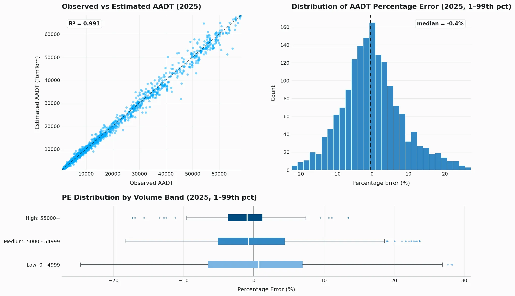
Belgium reaches the Good tier nationally (SQV 0.88) and holds it in every volume band, with a median percentage error below 0.5% and a tight, unbiased scatter in the AADT plot. Night-time hourly MAPE rises to 20.6%, but the corresponding MAE of roughly 29 vehicles shows the inflation stems from the low absolute volumes carried at night rather than from a loss of accuracy in absolute terms; the night SQV in fact improves to 0.91.
7.2 United Kingdom
AADT
| Road Category | Counters | MAPE (%) | 68th Pct APE (%) | 95th Pct APE (%) | Median PE (%) | SQV (15th Pct) |
|---|---|---|---|---|---|---|
| All roads | 6,465 | 4.0 | 4.3 | 12.4 | 0.0 | 0.90 |
| High (55,000+) | 1,961 | 2.3 | 2.6 | 6.4 | 0.1 | 0.90 |
| Medium (5,000–54,999) | 4,156 | 4.4 | 4.9 | 13.2 | -0.0 | 0.90 |
| Low (under 5,000) | 348 | 8.0 | 9.1 | 21.7 | 0.7 | 0.92 |
Hourly
Day hours (06:00–23:00)
| Road Category | Counters | MAE (veh/h) | MAPE (%) | 68th Pct APE (%) | 95th Pct APE (%) | Median PE (%) | SQV (15th Pct) |
|---|---|---|---|---|---|---|---|
| All roads | 6,326 | 104.0 | 7.7 | 6.6 | 17.8 | 0.0 | 0.89 |
| High (55,000+) | 1,935 | 145.8 | 6.1 | 4.8 | 10.9 | -0.2 | 0.88 |
| Medium (5,000–54,999) | 4,049 | 87.6 | 8.1 | 7.4 | 18.5 | 0.1 | 0.89 |
| Low (under 5,000) | 342 | 22.5 | 14.1 | 15.8 | 36.2 | 0.9 | 0.91 |
Night hours (23:00–06:00)
| Road Category | Counters | MAE (veh/h) | MAPE (%) | 68th Pct APE (%) | 95th Pct APE (%) | Median PE (%) | SQV (15th Pct) |
|---|---|---|---|---|---|---|---|
| All roads | 6,324 | 35.1 | 15.2 | 11.8 | 34.6 | -1.4 | 0.92 |
| High (55,000+) | 1,935 | 55.5 | 14.2 | 8.4 | 19.0 | -1.9 | 0.91 |
| Medium (5,000–54,999) | 4,049 | 26.4 | 14.7 | 13.3 | 35.3 | -1.0 | 0.92 |
| Low (under 5,000) | 340 | 7.2 | 31.6 | 33.3 | 95.0 | 0.0 | 0.93 |
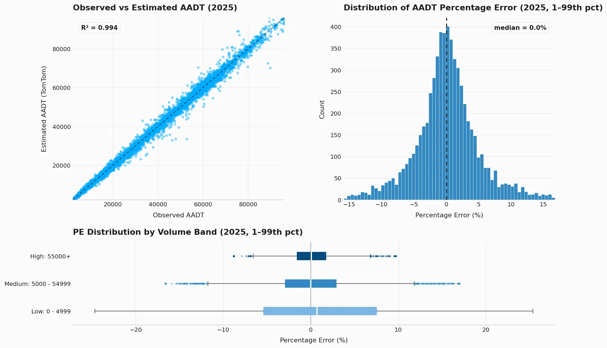
The United Kingdom delivers the strongest results in this assessment: the lowest national AADT MAPE (4.0%), an essentially unbiased median error, and a Very Good SQV of 0.90 or better sustained across all three volume bands. The high band is particularly accurate, with a MAPE of 2.3% and a 95th percentile APE of 6.4%. Hourly performance stays close to the AADT level during the day (MAPE 7.7%), and the night SQV remains Very Good at 0.92.
7.3 Netherlands
AADT
| Road Category | Counters | MAPE (%) | 68th Pct APE (%) | 95th Pct APE (%) | Median PE (%) | SQV (15th Pct) |
|---|---|---|---|---|---|---|
| All roads | 10,407 | 6.2 | 6.6 | 19.6 | -0.7 | 0.89 |
| High (55,000+) | 1,028 | 3.5 | 3.6 | 11.5 | -0.6 | 0.86 |
| Medium (5,000–54,999) | 7,280 | 5.7 | 6.0 | 17.9 | -0.8 | 0.88 |
| Low (under 5,000) | 2,099 | 9.5 | 11.1 | 25.8 | -0.8 | 0.92 |
Hourly
Day hours (06:00–23:00)
| Road Category | Counters | MAE (veh/h) | MAPE (%) | 68th Pct APE (%) | 95th Pct APE (%) | Median PE (%) | SQV (15th Pct) |
|---|---|---|---|---|---|---|---|
| All roads | 9,661 | 98.2 | 11.8 | 10.3 | 28.8 | -2.2 | 0.88 |
| High (55,000+) | 1,018 | 204.5 | 8.2 | 6.2 | 15.1 | -1.6 | 0.85 |
| Medium (5,000–54,999) | 6,689 | 101.5 | 10.8 | 9.4 | 24.1 | -2.1 | 0.87 |
| Low (under 5,000) | 1,954 | 24.6 | 17.8 | 18.5 | 42.4 | -4.0 | 0.91 |
Night hours (23:00–06:00)
| Road Category | Counters | MAE (veh/h) | MAPE (%) | 68th Pct APE (%) | 95th Pct APE (%) | Median PE (%) | SQV (15th Pct) |
|---|---|---|---|---|---|---|---|
| All roads | 9,653 | 29.2 | 17.7 | 17.7 | 50.0 | -2.7 | 0.92 |
| High (55,000+) | 1,018 | 71.4 | 10.3 | 9.9 | 23.8 | -1.0 | 0.90 |
| Medium (5,000–54,999) | 6,689 | 27.5 | 16.2 | 16.6 | 42.9 | -2.6 | 0.92 |
| Low (under 5,000) | 1,946 | 6.0 | 31.1 | 36.0 | 75.0 | -10.3 | 0.94 |
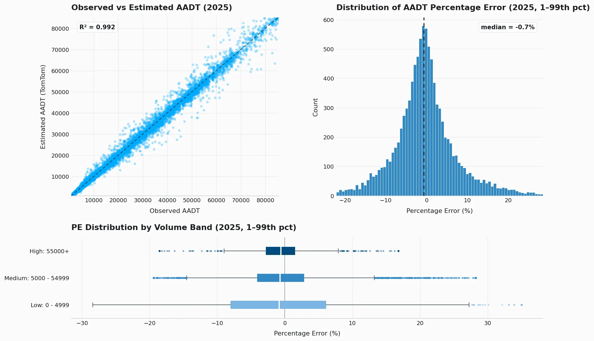
The Netherlands combines the largest counter sample in the document (10,407 loops) with consistently strong results, holding an SQV of at least 0.86 in every band and 0.89 nationally. A slight negative median percentage error recurs across all bands and in the hourly breakdown, indicating a mild systematic underestimation, though it remains below 1% at the AADT level. As elsewhere, night-time percentage errors are elevated while the night MAE of roughly 29 vehicles stays small and the night SQV reaches 0.92.
7.4 Norway
AADT
| Road Category | Counters | MAPE (%) | 68th Pct APE (%) | 95th Pct APE (%) | Median PE (%) | SQV (15th Pct) |
|---|---|---|---|---|---|---|
| All roads | 2,593 | 9.3 | 11.0 | 24.8 | -1.0 | 0.90 |
| High (55,000+) | 3 | 3.7 | 6.3 | 6.3 | -2.0 | 0.87 |
| Medium (5,000–54,999) | 1,161 | 8.3 | 9.7 | 22.4 | -1.4 | 0.87 |
| Low (under 5,000) | 1,429 | 10.2 | 12.1 | 26.1 | -0.3 | 0.92 |
Hourly
Day hours (06:00–23:00)
| Road Category | Counters | MAE (veh/h) | MAPE (%) | 68th Pct APE (%) | 95th Pct APE (%) | Median PE (%) | SQV (15th Pct) |
|---|---|---|---|---|---|---|---|
| All roads | 2,414 | 52.0 | 18.6 | 21.1 | 50.0 | 4.5 | 0.87 |
| High (55,000+) | 3 | 486.2 | 14.1 | 17.0 | 39.4 | 7.4 | 0.69 |
| Medium (5,000–54,999) | 1,124 | 77.5 | 16.0 | 18.1 | 43.1 | 5.3 | 0.85 |
| Low (under 5,000) | 1,287 | 26.5 | 21.1 | 24.1 | 55.2 | 3.3 | 0.89 |
Night hours (23:00–06:00)
| Road Category | Counters | MAE (veh/h) | MAPE (%) | 68th Pct APE (%) | 95th Pct APE (%) | Median PE (%) | SQV (15th Pct) |
|---|---|---|---|---|---|---|---|
| All roads | 2,336 | 13.1 | 28.9 | 32.6 | 75.0 | -3.6 | 0.92 |
| High (55,000+) | 3 | 49.7 | 11.3 | 13.5 | 27.1 | -0.1 | 0.88 |
| Medium (5,000–54,999) | 1,121 | 16.2 | 26.1 | 28.6 | 69.2 | -1.9 | 0.91 |
| Low (under 5,000) | 1,212 | 7.3 | 33.9 | 40.0 | 83.3 | -8.3 | 0.93 |
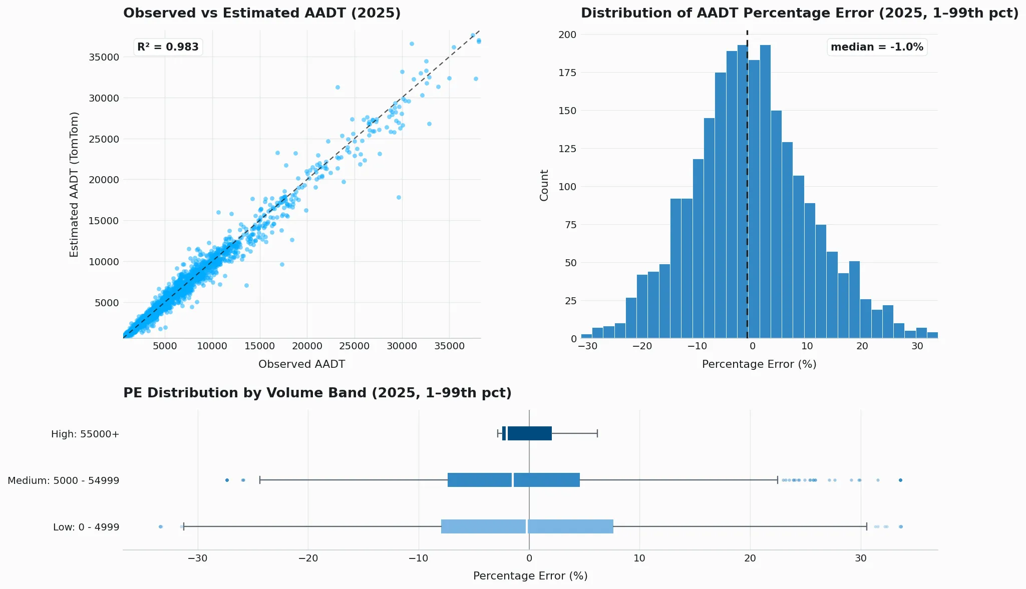
Norway posts one of the highest national AADT MAPE values in this assessment (9.3%) yet still achieves a Very Good SQV of 0.90, a pairing that indicates the percentage errors are inflated by the low absolute volumes that dominate the Norwegian network rather than by uncontrolled absolute errors. The high band contains only 3 counters, so its rows, including the below-threshold daytime hourly SQV of 0.69, rest on too small a sample to be conclusive. Night-time hourly MAPE reaches 28.9%, again a low-volume effect, with a night MAE of only about 13 vehicles.
7.5 New Zealand
AADT
| Road Category | Counters | MAPE (%) | 68th Pct APE (%) | 95th Pct APE (%) | Median PE (%) | SQV (15th Pct) |
|---|---|---|---|---|---|---|
| All roads | 527 | 10.0 | 11.6 | 25.7 | -2.0 | 0.87 |
| High (55,000+) | 21 | 5.8 | 6.9 | 15.6 | -2.6 | 0.82 |
| Medium (5,000–54,999) | 308 | 9.2 | 10.9 | 23.9 | -2.1 | 0.86 |
| Low (under 5,000) | 198 | 11.6 | 14.5 | 32.3 | -1.2 | 0.90 |
Hourly
Day hours (06:00–23:00)
| Road Category | Counters | MAE (veh/h) | MAPE (%) | 68th Pct APE (%) | 95th Pct APE (%) | Median PE (%) | SQV (15th Pct) |
|---|---|---|---|---|---|---|---|
| All roads | 516 | 65.4 | 16.3 | 18.2 | 43.4 | -1.5 | 0.87 |
| High (55,000+) | 20 | 265.1 | 8.1 | 9.8 | 20.6 | -3.5 | 0.80 |
| Medium (5,000–54,999) | 300 | 80.2 | 14.2 | 16.2 | 37.6 | -1.9 | 0.85 |
| Low (under 5,000) | 196 | 28.0 | 20.2 | 22.6 | 51.8 | 0.0 | 0.89 |
Night hours (23:00–06:00)
| Road Category | Counters | MAE (veh/h) | MAPE (%) | 68th Pct APE (%) | 95th Pct APE (%) | Median PE (%) | SQV (15th Pct) |
|---|---|---|---|---|---|---|---|
| All roads | 496 | 25.8 | 28.8 | 31.2 | 75.0 | -5.9 | 0.89 |
| High (55,000+) | 20 | 99.4 | 17.3 | 18.3 | 33.9 | -9.5 | 0.84 |
| Medium (5,000–54,999) | 292 | 26.1 | 27.4 | 30.0 | 70.5 | -5.0 | 0.89 |
| Low (under 5,000) | 184 | 9.1 | 35.4 | 38.9 | 100.0 | -7.3 | 0.92 |
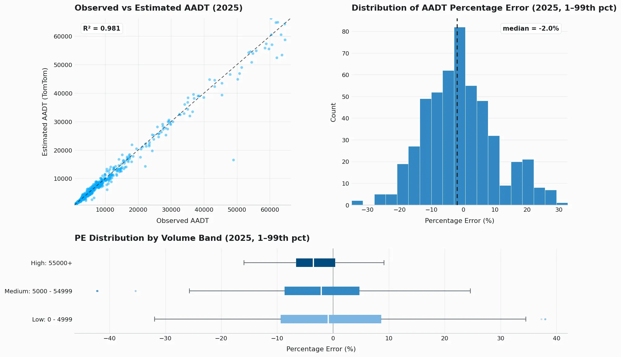
New Zealand carries the highest all-roads AADT MAPE in the document (10.0%) yet still reaches the Good tier (SQV 0.87), with its low band at Very Good (0.90). A mild negative median percentage error (-2.0% at the all-roads level) recurs in every volume band, the most pronounced under-prediction tendency of all countries in this assessment, although the AADT scatter remains tightly grouped around the diagonal apart from a single strong mid-volume outlier. The high band’s Acceptable SQV (0.82) rests on only 21 counters, too few for a stable estimate. Night-time hourly MAPE rises to 28.8% while the night MAE stays near 26 veh/h, the usual signature of low overnight volumes inflating percentage-based errors.
7.6 Sweden
AADT
| Road Category | Counters | MAPE (%) | 68th Pct APE (%) | 95th Pct APE (%) | Median PE (%) | SQV (15th Pct) |
|---|---|---|---|---|---|---|
| All roads | 618 | 7.8 | 8.8 | 24.3 | -0.4 | 0.85 |
| High (55,000+) | 24 | 4.8 | 5.5 | 15.3 | -1.8 | 0.80 |
| Medium (5,000–54,999) | 531 | 7.3 | 8.2 | 21.5 | -0.2 | 0.85 |
| Low (under 5,000) | 63 | 13.0 | 14.8 | 33.8 | -0.7 | 0.90 |
Hourly
Day hours (06:00–23:00)
| Road Category | Counters | MAE (veh/h) | MAPE (%) | 68th Pct APE (%) | 95th Pct APE (%) | Median PE (%) | SQV (15th Pct) |
|---|---|---|---|---|---|---|---|
| All roads | 544 | 115.9 | 11.3 | 11.3 | 30.4 | -0.6 | 0.85 |
| High (55,000+) | 24 | 244.9 | 7.7 | 8.0 | 19.0 | -2.0 | 0.81 |
| Medium (5,000–54,999) | 483 | 115.1 | 11.0 | 11.1 | 29.0 | -0.6 | 0.85 |
| Low (under 5,000) | 37 | 29.0 | 18.9 | 20.0 | 54.4 | 2.2 | 0.89 |
Night hours (23:00–06:00)
| Road Category | Counters | MAE (veh/h) | MAPE (%) | 68th Pct APE (%) | 95th Pct APE (%) | Median PE (%) | SQV (15th Pct) |
|---|---|---|---|---|---|---|---|
| All roads | 544 | 32.4 | 21.0 | 21.6 | 51.8 | -0.6 | 0.89 |
| High (55,000+) | 24 | 79.4 | 17.7 | 13.0 | 31.2 | -1.3 | 0.87 |
| Medium (5,000–54,999) | 483 | 31.1 | 20.5 | 21.6 | 50.0 | -0.8 | 0.89 |
| Low (under 5,000) | 37 | 6.8 | 34.0 | 37.5 | 100.0 | 3.2 | 0.93 |
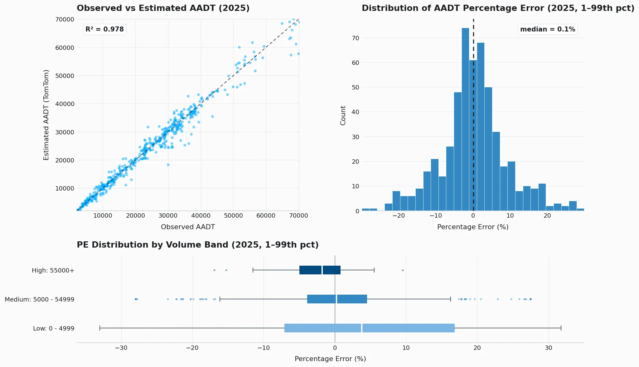
Sweden’s national SQV of 0.85 sits exactly on the Good threshold, and its high band lands on the Acceptable boundary at 0.80. With 618 counters, among the smallest samples in the document, and only 24 high-band and 63 low-band loops among them, the band-level results should be read as noisy rather than as stable estimates. The AADT scatter shows no material bias, with a median percentage error below 0.5% in magnitude.
7.7 United States
AADT
| Road Category | Counters | MAPE (%) | 68th Pct APE (%) | 95th Pct APE (%) | Median PE (%) | SQV (15th Pct) |
|---|---|---|---|---|---|---|
| All roads | 7,804 | 7.6 | 8.6 | 22.6 | 0.2 | 0.83 |
| High (55,000+) | 2,286 | 6.1 | 7.2 | 17.3 | 1.1 | 0.75 |
| Medium (5,000–54,999) | 4,105 | 7.7 | 8.6 | 23.3 | -0.2 | 0.85 |
| Low (under 5,000) | 1,413 | 9.8 | 11.2 | 27.3 | -0.4 | 0.92 |
Hourly
Day hours (06:00–23:00)
| Road Category | Counters | MAE (veh/h) | MAPE (%) | 68th Pct APE (%) | 95th Pct APE (%) | Median PE (%) | SQV (15th Pct) |
|---|---|---|---|---|---|---|---|
| All roads | 7,121 | 149.8 | 11.0 | 11.3 | 30.7 | 0.8 | 0.84 |
| High (55,000+) | 2,133 | 309.8 | 8.2 | 8.4 | 21.4 | 1.1 | 0.80 |
| Medium (5,000–54,999) | 3,692 | 96.3 | 10.9 | 11.5 | 29.8 | 0.5 | 0.86 |
| Low (under 5,000) | 1,296 | 21.8 | 16.9 | 18.6 | 45.2 | 0.3 | 0.91 |
Night hours (23:00–06:00)
| Road Category | Counters | MAE (veh/h) | MAPE (%) | 68th Pct APE (%) | 95th Pct APE (%) | Median PE (%) | SQV (15th Pct) |
|---|---|---|---|---|---|---|---|
| All roads | 7,103 | 53.8 | 16.8 | 17.5 | 50.0 | 0.6 | 0.89 |
| High (55,000+) | 2,132 | 118.8 | 11.0 | 11.5 | 31.2 | 1.8 | 0.85 |
| Medium (5,000–54,999) | 3,688 | 31.3 | 17.1 | 18.2 | 49.4 | 0.2 | 0.91 |
| Low (under 5,000) | 1,283 | 7.3 | 28.1 | 31.2 | 75.0 | 0.0 | 0.93 |
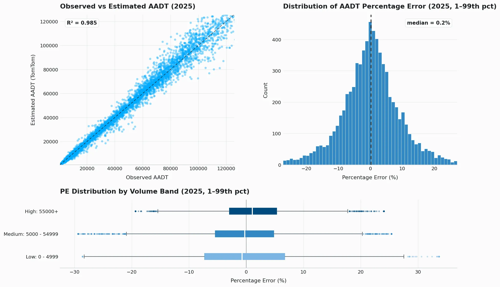
The United States records the lowest national SQV in the document (0.83, Acceptable), with the high band at 0.75 falling below the acceptance threshold while the low and medium bands stay at or above 0.85. Median percentage errors are small throughout, and the AADT scatter remains well centred on the diagonal. Hourly results follow the familiar day/night pattern, with the night SQV (0.89) above the daytime value (0.84) and the night MAPE inflation explained by low night volumes, the night MAE being roughly 54 vehicles against about 150 by day.
8. What the Results Mean for Your Use Case
8.1 For business decision-makers and analysts
Traffic volume data informs decisions at a strategic level: site viability, infrastructure priority, risk exposure, network performance. The question for most analytical applications is not whether the estimate is perfect, but whether the error range is acceptable for the decision at hand.
As a practical guide: a MAPE of 10% on a road carrying 20,000 vehicles per day means the estimate will typically be within 2,000 vehicles of the true figure. For retail site selection, insurance risk modeling, or transport infrastructure planning, this level of accuracy is consistent with, or better than, the accuracy delivered by traditional survey and estimation methods on comparable road types. For applications that require precise capacity calculations — such as junction design or traffic signal optimization — we recommend supplementing volume estimates with local count data where available and practicable.
Low-volume roads (under 5,000 vehicles per day) show higher MAPE values across all countries in this assessment. It is important to note that on roads with very low daily volumes, a higher percentage error typically represents a small number of vehicles in absolute terms. A MAPE of 15% on a road carrying 300 vehicles per day is a difference of approximately 45 vehicles — small in practical terms for most applications. For use cases that depend on individual low-volume rural roads, we recommend treating estimates as indicative and validating against available count data where precision is important.
8.2 For data scientists and transport modellers
The SQV 15th percentile is a conservative quality indicator. A stated SQV means that at least 85% of road segments in that category perform at or above the quality level shown. When integrating TomTom Historical Traffic Volumes into transport models, the SQV provides guidance on which road categories can be used with confidence and where additional validation against local counts is advisable.
For road categories showing SQV values at or above 0.80 (Acceptable), the data is suitable for use in transport models and analytical workflows requiring segment-level accuracy. For categories below 0.80, treat the data as indicative and apply additional quality filters or local calibration where precision is required.
The Median Percentage Error (bias) values from this assessment are generally small and, for most categories, close to zero. This means that aggregate measures — such as total vehicle kilometres travelled across a network, or average AADT for a road class — will be reliable, even where individual segment errors exist. The systematic negative bias on medium and high-volume roads in several countries (indicating a slight tendency to under-predict) should be accounted for in applications where absolute volume totals are important.
9. Summary
This paper presents a transparent account of the accuracy of TomTom Historical Traffic Volumes for 2025, based on k-fold cross-validation against independent ground-truth counts across seven countries.
In the 2025 assessment the United Kingdom leads with an all-roads AADT MAPE of 4.0% and a Very Good SQV in every volume band, and six of the seven countries keep their all-roads MAPE below 10%. Median percentage errors remain small throughout, so aggregate network-level measures can be used with confidence.
New Zealand pairs the highest national MAPE (10.0%) with a Good SQV of 0.87, indicating errors that remain well-controlled in absolute terms; readers using segment-level data should consult the band-level tables and the guidance in Section 8.2.
For low-volume roads, MAPE values are higher across all countries in percentage terms. The absolute difference in vehicle count on these roads is typically small, and the results should be interpreted in that context.
For markets beyond the seven countries in this k-fold validation, Leave-One-Country-Out (LOCO) validation — described in Section 6 — provides the accuracy basis.
TomTom is committed to transparent reporting of model performance, including where results fall short of quality thresholds. This paper is intended to give customers the information they need to use TomTom Historical Traffic Volumes data with confidence, informed by a clear understanding of both its accuracy and its limitations.
10. References
Friedrich, M., Pestel, E., Schiller, C., & Simon, R. (2019). Scalable GEH: A Quality Measure for Comparing Observed and Modeled Single Values in a Travel Demand Model Validation. Transportation Research Record, 2673(4), 722–732. https://doi.org/10.1177/0361198119838849