
AADT Accuracy and Validation 2024
1. Executive summary
This document reports the accuracy of the TomTom Historical Traffic Volumes annual averages, AADT and AAWHT, for 2024. Sections 2 to 6 describe the product and how we validate it and are the same in every year’s document; Section 7 and the key findings below are specific to 2024.
We measured accuracy against independent ground-truth traffic counts from permanent loop detectors and similar counting infrastructure in seven countries (Australia, Belgium, Netherlands, Norway, Sweden, United Kingdom, and United States) for 2024. The per-country metrics in this document come from k-fold cross-validation, which tests the model on data it was not trained on (Section 5). For markets beyond these seven countries, Section 6 describes the complementary leave-one-country-out (LOCO) validation, whose pooled results for 2024 are reported in Section 7.8. A market is a country where the product is available.
Key findings:
- The United Kingdom is the strongest performer in this assessment, with an all-roads AADT MAPE of 4.8% and a near-perfect high-volume band (MAPE 2.1%, SQV 0.91, Very good).
- Across the seven countries, all-roads AADT MAPE ranges from 4.8% (United Kingdom) to 9.7% (Norway); Norway pairs the highest MAPE of the group with its strongest quality score (SQV 0.91, Very good), showing that errors remain well-controlled in absolute terms.
- Sweden shows the widest error spread of the group, with a 95th percentile APE above 30% on the smallest national sample in this assessment (855 counters), although its all-roads MAPE of 8.3% is in line with the other countries.
- For markets without local counter data, the pooled leave-one-country-out results (Section 7.8) give an all-roads AADT MAPE of 12.9%, above every k-fold country in this assessment; the SQV of 0.76 is Acceptable overall while low-volume roads stay Good (0.89).
- Percentage errors are consistently higher on low-volume roads in every country, but on such roads they correspond to small absolute vehicle counts; Section 8 provides guidance on interpreting these values.
2. Introduction
How many vehicles pass a road segment on a typical day, and at a typical hour of the week? TomTom Historical Traffic Volumes estimates exactly that, for each road segment. We apply machine learning to probe data: the position and speed reports that millions of connected vehicles send (Sekuła et al., 2018; Zhan et al., 2017). The annual averages cover most roads of the network.
Historical Traffic Volumes delivers three quantities: AADT, AAWHT and hourly volumes. The product introduction defines them. This document covers AADT and AAWHT; the hourly volumes are documented in the Hourly volumes section of this documentation.
We improve the model continuously, and an improved model can recompute past periods, so a published figure for a past period can improve after publication (Section 9).
Traffic volume data informs decisions with real consequences:
- Where to open a new store
- How to allocate infrastructure budgets
- How to assess road safety risk
- Whether the surrounding road network can support a proposed development
- Whether a new lane, a closure or another change to a road altered traffic, comparing the period before with the period after
Every one of those decisions rests on a volume number, so the useful question is not whether the data is reliable but how far off it can be on the roads you care about. This document answers that in vehicles, in percentages and as quality scores.
Traditional counting methods give precise counts at a small number of fixed points (Federal Highway Administration, 2022). TomTom Historical Traffic Volumes estimates the volume across the road network of a covered market. An estimate carries uncertainty, so we measure that uncertainty with the metrics defined in Section 4. With those numbers, customers can decide where and how to use the data.
We validate against counters: permanent loop detectors and similar counting stations whose independent ground-truth counts played no part in model training. The accuracy metrics in this document measure the gap between our estimates and those reference counts; a smaller gap means a more accurate estimate. Where results fall short of the quality thresholds in Section 4.4, we say so and give the available context.
3. How the model works
Turning raw reports from connected vehicles into reliable, network-wide volume estimates takes a sequence of steps, and each step solves a distinct problem. Unlike traditional counting methods, the product needs no physical equipment at each measurement point. We collect probe observations (Section 3.1), estimate the penetration rate (Section 3.2) and convert probe observations into volume estimates (Section 3.3). Section 3.4 describes the two annual averages the model produces.
3.1 From connected vehicles to traffic observations
Our primary data source is floating-car data: GPS and telematics signals from connected vehicles (Herrera et al., 2010). Each signal is a probe observation; together, the signals form the probe data. Connected vehicles include:
- In-vehicle navigation systems
- Smartphones running navigation apps
- Connected commercial vehicles
The signals arrive passively and continuously from millions of devices worldwide. For each road segment, they form a continuous stream of speed and passage observations.
Probe observations are not traffic volumes, though. Only a fraction of the vehicles on a given road are connected and contributing data. We call this fraction the penetration rate. It varies by road type, geography and time of day, so converting probe observations into total volume estimates means accounting for that variation.
3.2 Estimating the penetration rate without counters
A probe count becomes a traffic volume only once we know the penetration rate: the share of vehicles on that road that report probe data. Permanent counters measure it directly, but they exist on a small fraction of roads, and in many markets on none. A method that needs counters everywhere cannot scale. Ours needs them only once, to learn.
The key is congestion. When a road operates at or near capacity (Transportation Research Board, 2022), physics constrains it: the relationship between the speed vehicles drive and the number of vehicles the road carries becomes tight and predictable, as the fundamental diagram of traffic flow describes (Greenshields, 1935; Treiber & Kesting, 2013). From probe speeds, read together with the road’s attributes, we can then estimate how many vehicles the road carries. We train a capacity model on roads with counters to learn this speed-to-flow relationship, together with map attributes such as road class, urban or rural context and lane configuration. Because the same congestion physics applies wherever a road runs near capacity (Kerner, 2004), the model transfers to roads that have never had a counter.
On any congested road we then hold two independent numbers: the total flow the capacity model estimates from speeds, and the probe flow we count directly. Their ratio is the penetration rate. Wherever probes meet congestion, we obtain a penetration-rate estimate, far beyond counter locations (Eisinga & Lorkowski, 2025). Individual estimates are noisy, so we aggregate them by region and road type into summaries that resist noise and fill the remaining gaps from similar surroundings. The result is a consistent picture of probe representativeness across countries and road classes. Roads that never congest inherit the estimate of their region and road type.
3.3 From penetration rate to traffic volume
The regional penetration picture tells us roughly what share of traffic the probes capture around a road. The volume model turns that into an estimate for the specific road. We train it on real ground truth: permanent counters, where they exist. From those counts it learns how the regional penetration rate, the observed probe data and the road’s own attributes combine into the volume of one road, in effect refining the regional penetration rate down to each segment. Once trained, it needs no counters. It runs wherever probe data and a map exist, which is what makes the product scalable to new regions, and why Section 6 tests it on countries it has never seen.
A motorway and a residential street sit at opposite ends of a wide range: among the counters the model learns from, the quietest carry fewer than 500 vehicles a day and the busiest more than 125,000. The relationship between a road’s attributes, its probe activity and its traffic load is not the same at the two ends. The estimate has to hold across that whole range, not only for the average road. So we train the model on counters across the full range of volumes, and we judge it on the same range. Section 7 reports its accuracy separately for high-, medium- and low-volume roads in every validated country, in the volume categories Section 5 defines. A reader can see where the estimates are strong and where they are weaker rather than take our word for it.
The model is tested only against counters it did not learn from. In k-fold cross-validation (Section 5), each counter is scored by a training round that did not include it. In leave-one-country-out validation (Section 6), a whole country is removed from training and scored as if it were a new market. Expect lower accuracy in a country the model has never seen than in one whose counters it trained on. Section 7.8 shows the difference for 2024; for markets without counters, it is the accuracy basis.
The two ends of the range err in different ways, and the metrics in Section 4 are chosen to show both. On a quiet road a handful of vehicles is a large share of the count, so percentage errors tend to be largest on low-volume roads even where the error in vehicles is small (Das & Tsapakis, 2020; Section 4.1). On a busy road the same percentage means many more vehicles. The Scalable Quality Value (Section 4.4) scales the error to the size of the count, so the two ends can be compared on one score. The median percentage error (Section 4.2) shows whether the estimates in a category lean high or low.
The volume model produces the two annual averages, AADT and AAWHT (Section 3.4).
3.4 What we publish: AADT and AAWHT
AADT, annual average daily traffic, is one value per road segment and year: the number of vehicles that pass the segment on an average day of that year. It is the standard yardstick of transport planning and the basis of network-wide totals such as vehicle kilometers traveled.
AAWHT, annual average week-hour traffic, is 168 values per segment and year in vehicles per hour, one for each hour of each day of the week: the typical Tuesday between 8am and 9am, for example. It describes the weekly rhythm of a road: the morning and evening peaks, the quiet of the night, the difference between a weekday and a Sunday.
The two are one profile at two resolutions. Summing the 24 AAWHT values of a day gives the typical volume of that day of the week, and the mean over the seven days gives the AADT. The hourly volumes documented in the Hourly volumes section are produced by starting from the typical value for that road, that day of the week and that hour, and adjusting it by how busy the road was in the period being estimated, as observed in probe data.
4. How we measure accuracy
One number cannot show both the typical error and its spread, so we report a set of complementary metrics. Each one highlights a different aspect of performance, and every one is measured against independent ground-truth counts. For AADT, each counter contributes one value per year; for AAWHT, one value for each of its 168 week-hours (Section 5 explains both).
| Metric | What it measures |
|---|---|
| MAPE (Mean Absolute Percentage Error) | The average percentage by which estimates differ from actual counts, regardless of direction. The primary summary measure. Lower is better. |
| Median Percentage Error | The middle value of all signed errors. Indicates systematic bias: positive = tendency to over-predict; negative = tendency to under-predict. Values close to zero are ideal. |
| 68th and 95th Percentile APE | The spread of errors across road segments. The 68th percentile covers roughly one standard deviation; the 95th captures the tail of the distribution where the model is most challenged. |
| SQV (Scalable Quality Value, 15th Pct) | A bounded quality score (0 to 1) designed to be consistent across roads of all volumes. Reported at the 15th percentile: at least 85% of segments perform better than this value. |
4.1 Mean absolute percentage error (MAPE)
MAPE measures the average size of the prediction error relative to the observed count, as a percentage. A MAPE of 10% means that estimates differ from actual counts by 10% on average. MAPE treats errors of all sizes equally, and it is a commonly reported accuracy measure in traffic estimation.
On very low-volume roads, a high percentage error can mean a small difference in vehicles (Hyndman & Koehler, 2006). A road with 300 vehicles per day and a MAPE of 15% has a typical absolute error of roughly 45 vehicles. For most planning and analytical purposes, a difference of that size is negligible. So read MAPE values for low-volume roads alongside the absolute volumes that matter for your use case.
4.2 Median percentage error
The median percentage error is the middle value of all signed errors: positive when our estimate exceeds the actual count, negative when it falls short. A value close to zero shows that the model has no strong tendency to over- or under-count. Low bias matters for applications such as aggregated network analysis or vehicle kilometers traveled (VKT) calculations, because systematic errors add up across many road segments.
4.3 68th and 95th percentile absolute percentage error
These percentiles describe how the errors spread across road segments. The 68th percentile corresponds roughly to one standard deviation in a normal distribution: about 68% of segments have an error at or below it. The 95th percentile captures the upper range, the error level of the most challenging segments. Together with MAPE, the percentiles show how the error is distributed, not only its average.
4.4 Scalable Quality Value (SQV)
A percentage error looks large on a quiet road and an absolute error looks large on a busy one. The Scalable Quality Value (Friedrich et al., 2019) handles both cases. It generalizes the GEH statistic used in transport model validation (Department for Transport, 2026). It is a bounded, scale-independent quality metric with a score between 0 and 1, where 1 is a perfect match. It measures the error against a yardstick that grows with the square root of the count, so it tolerates a larger percentage error on quiet roads, where a few vehicles make a large percentage, and a larger absolute error on busy roads. It then maps the result to a bounded score. SQV is therefore consistent across the full range of traffic volumes. The formula is
SQV = 1 / (1 + sqrt((M − C)² / (f × C)))
where M is the modeled value, C is the observed count and f is a scaling factor set by the order of magnitude of the quantity: 10,000 for daily volumes such as AADT and 1,000 for hourly volumes such as AAWHT. An error of zero gives a score of 1; the larger the error relative to the count, the lower the score. For example, an AADT estimate of 11,000 vehicles against a count of 10,000 scores about 0.91, and so does an AAWHT estimate of 1,100 vehicles in an hour against a count of 1,000. We report SQV as its 15th percentile across all segments in each group: at least 85% of the road segments in the group perform better than the stated value. The quality thresholds below come from Friedrich et al. (2019):
| SQV | Assessment | Guidance for use |
|---|---|---|
| ≥ 0.90 | Very good | High confidence in segment-level comparisons. Suitable for precision analytics and granular planning. |
| ≥ 0.85 | Good | Suitable for cross-segment analysis and most planning applications. |
| ≥ 0.80 | Fair | Suitable for network-level planning and transport modeling. Validate individual segments where precision matters. |
| ≥ 0.75 | Acceptable | Suitable for aggregate and indicative use. Validate against local count data before relying on individual segments. |
| Below 0.75 | Insufficient | Use with caution. Treat results as indicative and validate against local count data where possible. |
5. Validation approach: K-fold cross-validation
The per-country accuracy metrics in this document come from k-fold cross-validation. The method tests the model on data it was not trained on, which gives a realistic measure of real-world performance.
We divide the counter-equipped road segments used in training into five groups, called folds (Roberts et al., 2017). In each round, we hold one fold back entirely, train the model on the remaining folds and evaluate it against the held-back segments. This repeats until every fold has served as the test set. We then aggregate the accuracy figures across all rounds, so every validation counter contributes to the reported results without ever training the model it is evaluated against.
The same rounds validate both annual averages. For AADT, each held-back counter contributes one value per year: its AADT estimate against the AADT derived from its counts. For AAWHT, it contributes one value per week-hour: the estimate for that hour of the week against the counter’s average for it over the year, so the AAWHT metrics are computed across segment-hours. Counters without usable hourly data are left out of the AAWHT figures, so the counter numbers in the AADT and AAWHT tables of Section 7 can differ slightly.
K-fold cross-validation is standard practice in machine learning (Hastie et al., 2009): it prevents overfitting to one test set, uses all available ground-truth data and gives a reliable estimate of how well the model generalizes.
We report results for three volume categories. The volume category is a different grouping from road class, the functional class of a road in the map, such as motorway, major road or local street:
- High-volume roads: 55,000 or more vehicles per day (AADT)
- Medium-volume roads: 5,000–54,999 vehicles per day
- Low-volume roads: fewer than 5,000 vehicles per day
An All roads row gives the aggregated metrics across all counters, regardless of volume category. Section 7 reports the AADT and AAWHT results for each country and, in Section 7.8, pooled for countries held out from training.
K-fold cross-validation needs ground-truth counting data for every country in the validation set. For markets without counter data, Section 6 describes the complementary leave-one-country-out (LOCO) approach we use to estimate accuracy.
6. Leave-one-country-out (LOCO) validation
TomTom Historical Traffic Volumes is available in many markets with no permanent counting infrastructure. K-fold cross-validation (Section 5) needs ground-truth data, so it cannot be applied directly there. Leave-one-country-out (LOCO) validation fills that gap: in countries that do have counters, it measures how the model performs in a country it has never seen, and uses that result as the accuracy estimate for a market without counters (Roberts et al., 2017). This transfer assumes that the held-out countries resemble the unseen market in road network structure and probe coverage.
6.1 How LOCO validation works
In LOCO validation, we exclude one country entirely from model training. We train the model on all remaining countries and then evaluate it against the held-out country with the counter data available there. This repeats for each country in turn, so every country serves once as an unseen test market. We report the results jointly for the held-out countries in a year rather than per country, so they describe the accuracy to expect in a market the model has never seen, not the accuracy of any one country.
LOCO simulates deployment in a market where the model has never seen local data. Its results therefore estimate performance in new markets, where the model relies entirely on what it has learned from other countries.
6.2 Why LOCO matters for customers
If you use TomTom Historical Traffic Volumes in a market beyond the seven countries in Section 7, the LOCO results in Section 7.8 are your primary quality basis. The model learns traffic patterns that carry across countries: road network structure, speed-flow relationships, penetration-rate dynamics. Those learned patterns are what the model carries into a market it has never seen. The LOCO results show how much of its accuracy travels with them.
6.3 Where the LOCO results are reported
The LOCO results for 2024 are reported in Section 7.8, next to the per-country k-fold results and in the same tables and metrics, pooled across the countries held out from training. Because the held-out countries are evaluated jointly, the figures describe the accuracy to expect in a market the model has never seen rather than any specific market. They extend the k-fold results in Section 7 to every market where the product is available. The pooled AAWHT figures are computed in the hourly evaluation and cover a larger set of held-out counters than the pooled AADT figures, which is why their counter numbers differ.
7. Results (2024)
The tables below give the AADT and AAWHT accuracy results for each of the seven countries in the 2024 k-fold validation, followed by the pooled leave-one-country-out (LOCO) results for countries held out from training (Section 6). Section 4.4 defines the quality tiers for the SQV (15th Pct) values.
7.1 Australia
AADT
| Road Category | Counters | MAPE (%) | 68th Pct APE (%) | 95th Pct APE (%) | Median PE (%) | SQV (15th Pct) |
|---|---|---|---|---|---|---|
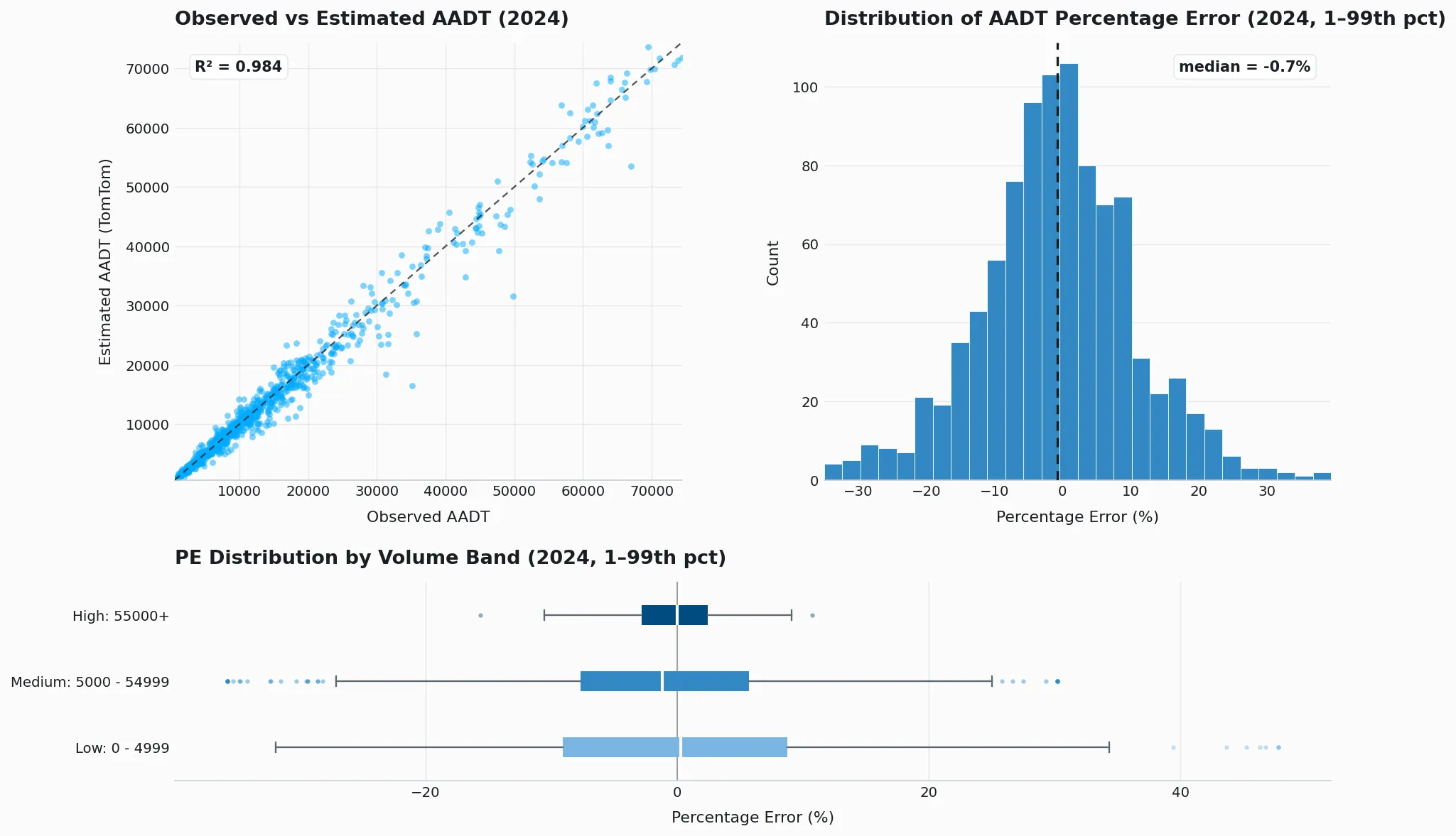
| All roads | 970 | 9.5 | 10.7 | 28.2 | -0.8 | 0.85 |
| High (55,000+) | 48 | 3.8 | 4.2 | 10.6 | 0.0 | 0.85 |
| Medium (5,000–54,999) | 663 | 9.3 | 10.5 | 27.1 | -1.2 | 0.83 |
| Low (under 5,000) | 259 | 11.3 | 11.9 | 34.4 | -0.1 | 0.91 |
AAWHT
| Road Category | Counters | MAPE (%) | SQV (15th Pct) |
|---|---|---|---|
| All roads | 898 | 12.0 | 0.87 |
| High (55,000+) | 42 | 5.5 | 0.86 |
| Medium (5,000–54,999) | 619 | 11.6 | 0.86 |
| Low (under 5,000) | 237 | 14.7 | 0.91 |
Australia posts a Good overall SQV (0.85) with an essentially unbiased error distribution (median PE -0.8%), and its high-volume band is notably strong at 3.8% MAPE, albeit from a small sample of 48 counters. Unusually, the medium band is the country’s weakest (SQV 0.83, Fair), sitting below both the low and high bands.
7.2 Belgium
AADT
| Road Category | Counters | MAPE (%) | 68th Pct APE (%) | 95th Pct APE (%) | Median PE (%) | SQV (15th Pct) |
|---|---|---|---|---|---|---|
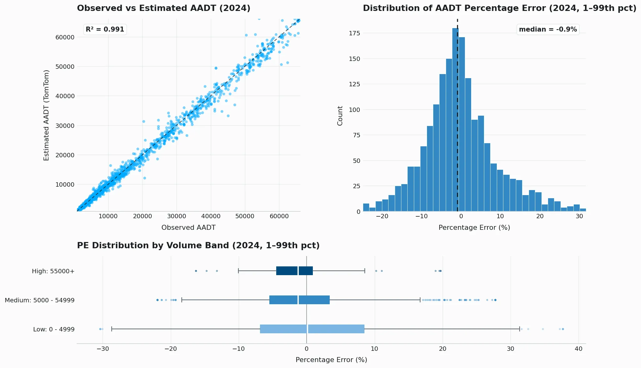
| All roads | 1,833 | 7.7 | 8.6 | 22.7 | -1.0 | 0.88 |
| High (55,000+) | 113 | 4.6 | 4.7 | 18.0 | -1.1 | 0.83 |
| Medium (5,000–54,999) | 1,157 | 6.8 | 7.4 | 20.3 | -1.2 | 0.87 |
| Low (under 5,000) | 563 | 10.0 | 12.1 | 28.0 | 0.0 | 0.91 |
AAWHT
| Road Category | Counters | MAPE (%) | SQV (15th Pct) |
|---|---|---|---|
| All roads | 1,789 | 9.4 | 0.89 |
| High (55,000+) | 112 | 6.1 | 0.83 |
| Medium (5,000–54,999) | 1,130 | 8.5 | 0.89 |
| Low (under 5,000) | 547 | 12.4 | 0.93 |
Belgium posts solid mid-pack AADT accuracy (MAPE 7.7%, SQV 0.88) with a near-symmetric error distribution and Good-or-better SQV across all three volume bands.
7.3 Netherlands
AADT
| Road Category | Counters | MAPE (%) | 68th Pct APE (%) | 95th Pct APE (%) | Median PE (%) | SQV (15th Pct) |
|---|---|---|---|---|---|---|
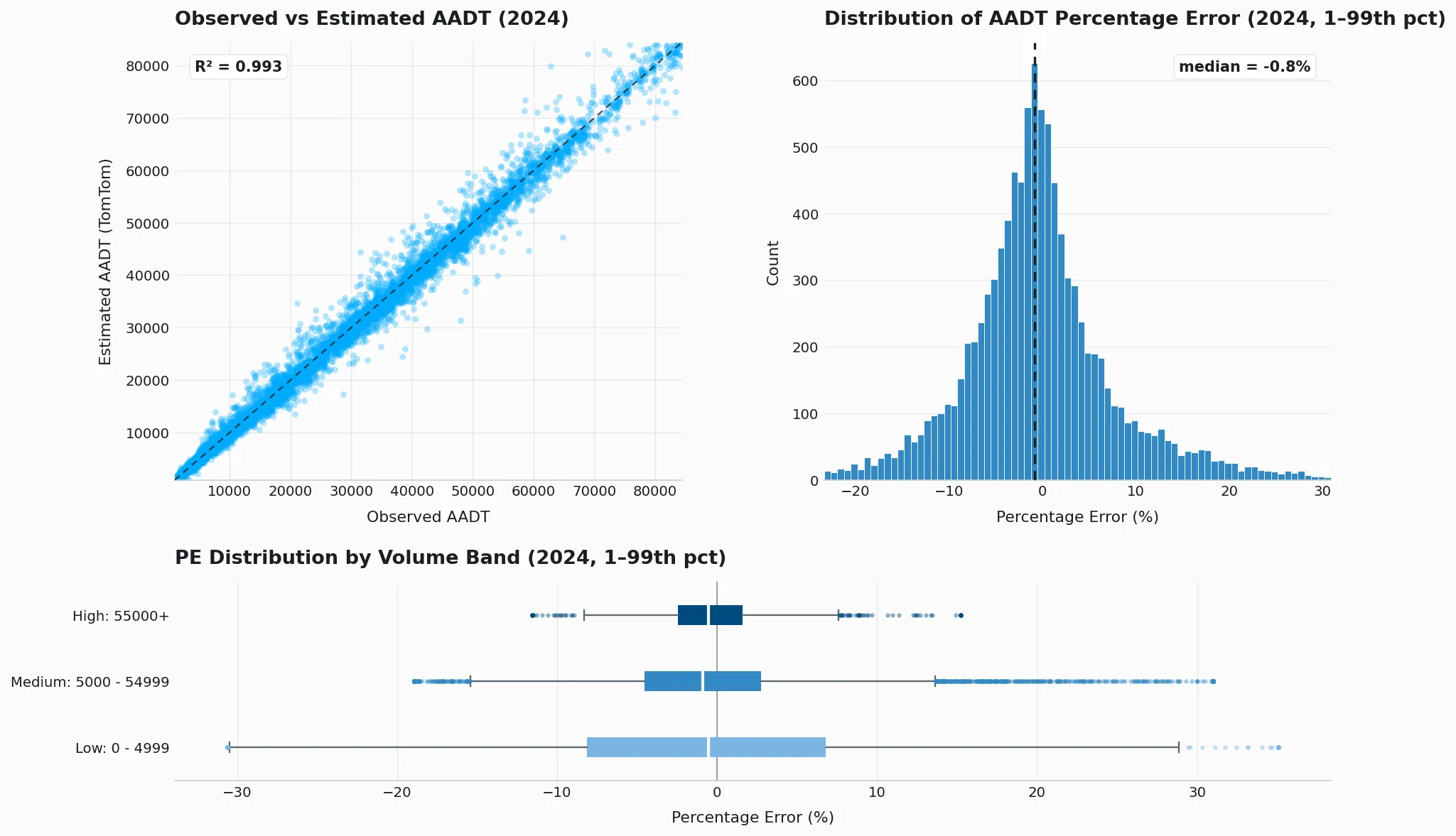
| All roads | 10,379 | 6.4 | 6.9 | 20.1 | -0.8 | 0.88 |
| High (55,000+) | 1,023 | 3.1 | 3.2 | 9.3 | -0.5 | 0.87 |
| Medium (5,000–54,999) | 7,307 | 5.9 | 6.3 | 18.2 | -0.9 | 0.88 |
| Low (under 5,000) | 2,049 | 10.0 | 11.9 | 26.4 | -0.5 | 0.91 |
AAWHT
| Road Category | Counters | MAPE (%) | SQV (15th Pct) |
|---|---|---|---|
| All roads | 10,151 | 7.7 | 0.90 |
| High (55,000+) | 1,020 | 3.9 | 0.89 |
| Medium (5,000–54,999) | 7,132 | 7.1 | 0.89 |
| Low (under 5,000) | 1,999 | 12.4 | 0.92 |
The Netherlands turns in consistently strong results (MAPE 6.4%, SQV 0.88) with every volume band at Good or above and only a slight under-prediction bias (median PE −0.8%).
7.4 Norway
AADT
| Road Category | Counters | MAPE (%) | 68th Pct APE (%) | 95th Pct APE (%) | Median PE (%) | SQV (15th Pct) |
|---|---|---|---|---|---|---|
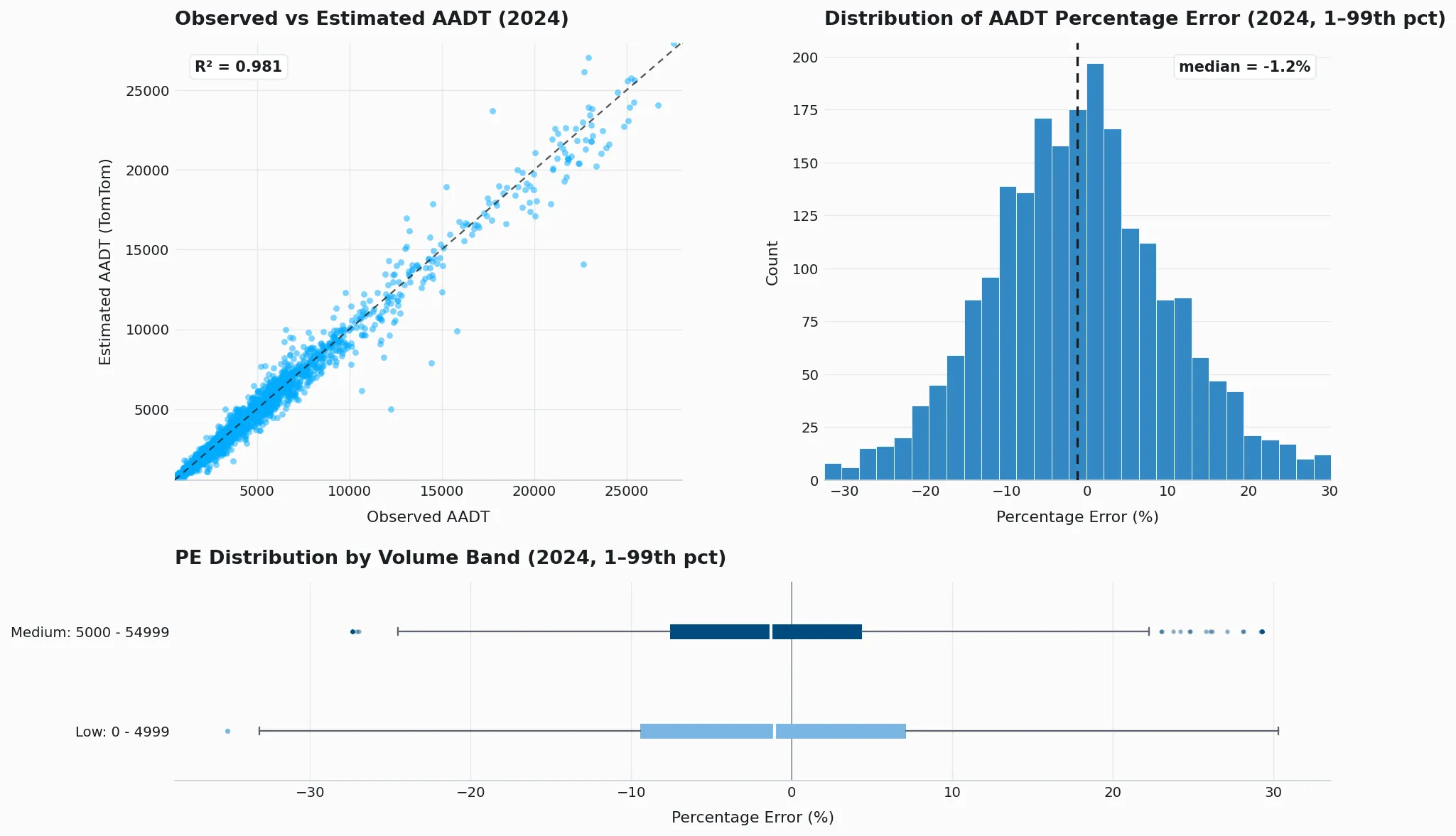
| All roads | 2,334 | 9.7 | 11.6 | 25.8 | -1.2 | 0.91 |
| Medium (5,000–54,999) | 801 | 8.3 | 9.8 | 23.0 | -1.2 | 0.88 |
| Low (under 5,000) | 1,533 | 10.5 | 12.5 | 26.7 | -1.1 | 0.92 |
AAWHT
| Road Category | Counters | MAPE (%) | SQV (15th Pct) |
|---|---|---|---|
| All roads | 2,199 | 12.1 | 0.91 |
| Medium (5,000–54,999) | 785 | 10.2 | 0.90 |
| Low (under 5,000) | 1,414 | 13.4 | 0.92 |
Norway achieves the highest base SQV of all countries in this assessment (0.91, Very good) even though its MAPE (9.7%) is mid-to-high — a pairing that shows errors remain well-controlled in absolute terms. It has no high-volume band, as the country has no counters above 55,000 AADT, so quality is reported for the low and medium bands only, both Good or better.
7.5 Sweden
AADT
| Road Category | Counters | MAPE (%) | 68th Pct APE (%) | 95th Pct APE (%) | Median PE (%) | SQV (15th Pct) |
|---|---|---|---|---|---|---|
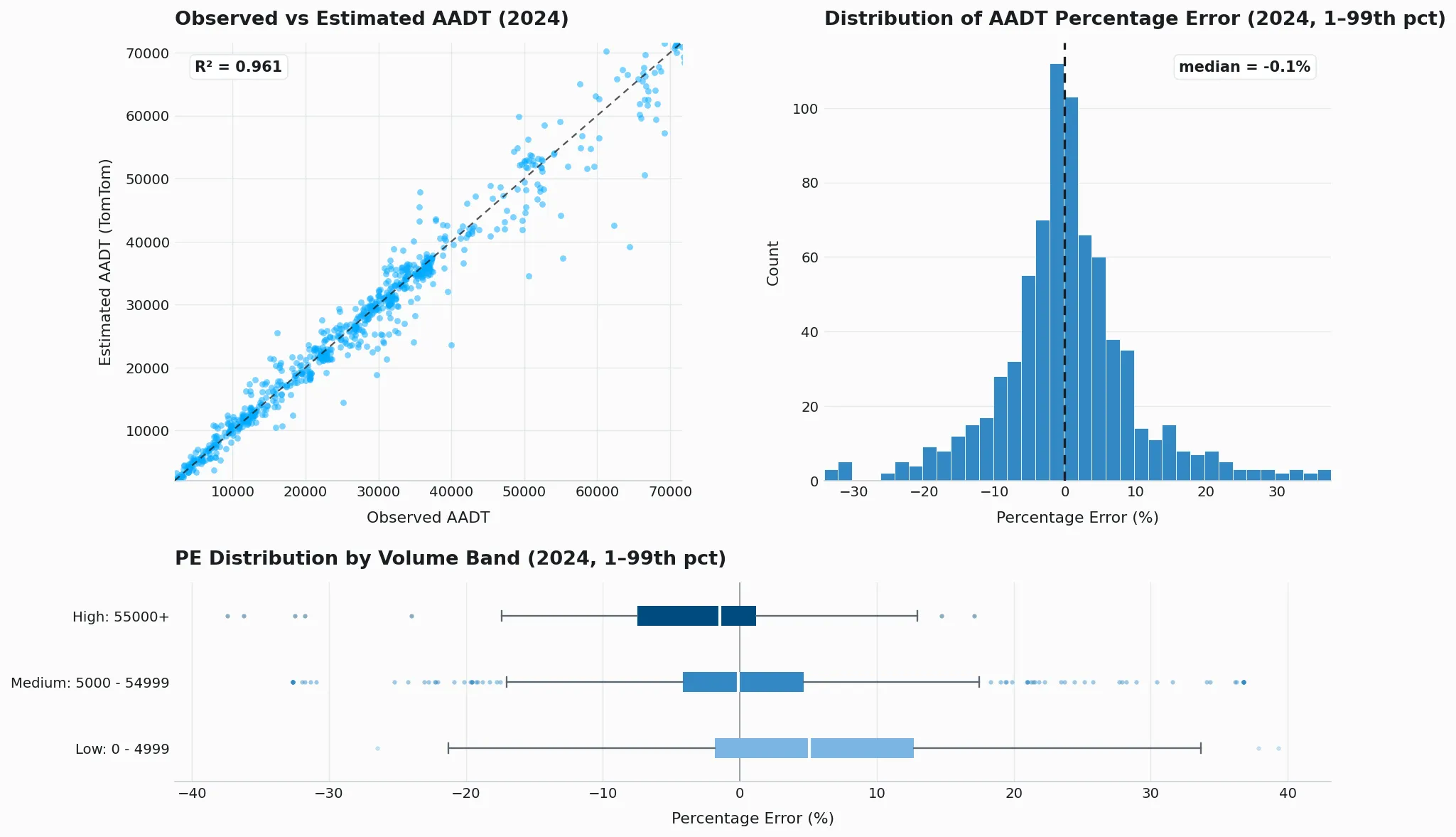
| All roads | 855 | 8.3 | 8.4 | 30.9 | -0.3 | 0.82 |
| High (55,000+) | 60 | 7.7 | 7.3 | 31.7 | -1.5 | 0.75 |
| Medium (5,000–54,999) | 731 | 7.7 | 7.8 | 25.8 | -0.4 | 0.82 |
| Low (under 5,000) | 64 | 15.0 | 18.0 | 41.1 | 6.4 | 0.86 |
AAWHT
| Road Category | Counters | MAPE (%) | SQV (15th Pct) |
|---|---|---|---|
| All roads | 782 | 9.5 | 0.85 |
| High (55,000+) | 60 | 8.1 | 0.80 |
| Medium (5,000–54,999) | 667 | 9.2 | 0.86 |
| Low (under 5,000) | 55 | 14.8 | 0.91 |
Sweden is the weakest AADT performer, with the lowest base SQV (0.82, Fair) and the widest upper error tail (95th-percentile APE above 30%), on the smallest national sample in this assessment (855 counters). Its high band is Acceptable (SQV 0.75) and its low band carries an elevated MAPE (15%), but both rest on very sparse samples (60 and 64 counters respectively), too few for stable estimates.
7.6 United Kingdom
AADT
| Road Category | Counters | MAPE (%) | 68th Pct APE (%) | 95th Pct APE (%) | Median PE (%) | SQV (15th Pct) |
|---|---|---|---|---|---|---|
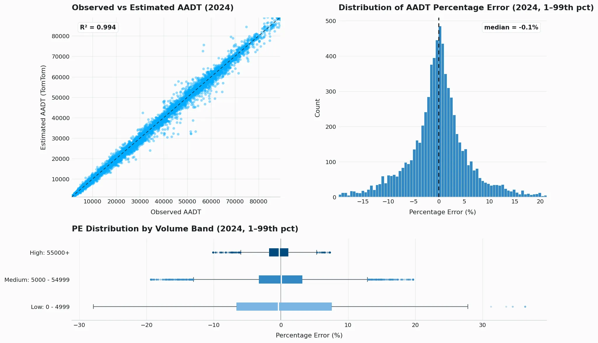
| All roads | 7,298 | 4.8 | 5.0 | 15.5 | -0.1 | 0.89 |
| High (55,000+) | 1,725 | 2.1 | 2.3 | 6.3 | -0.2 | 0.91 |
| Medium (5,000–54,999) | 4,888 | 5.0 | 5.6 | 15.2 | 0.0 | 0.89 |
| Low (under 5,000) | 685 | 9.5 | 11.3 | 25.7 | -0.5 | 0.92 |
AAWHT
| Road Category | Counters | MAPE (%) | SQV (15th Pct) |
|---|---|---|---|
| All roads | 7,175 | 5.8 | 0.91 |
| High (55,000+) | 1,724 | 2.9 | 0.92 |
| Medium (5,000–54,999) | 4,805 | 5.9 | 0.90 |
| Low (under 5,000) | 646 | 12.0 | 0.93 |
The United Kingdom is the strongest AADT performer in the document, with the lowest MAPE (4.8%) and the tightest error spread of all countries in this assessment; its scatter is essentially unbiased (median PE −0.1%). All three bands reach Good or Very good, the high band being near-perfect (MAPE 2.1%, SQV 0.91).
7.7 United States
AADT
| Road Category | Counters | MAPE (%) | 68th Pct APE (%) | 95th Pct APE (%) | Median PE (%) | SQV (15th Pct) |
|---|---|---|---|---|---|---|
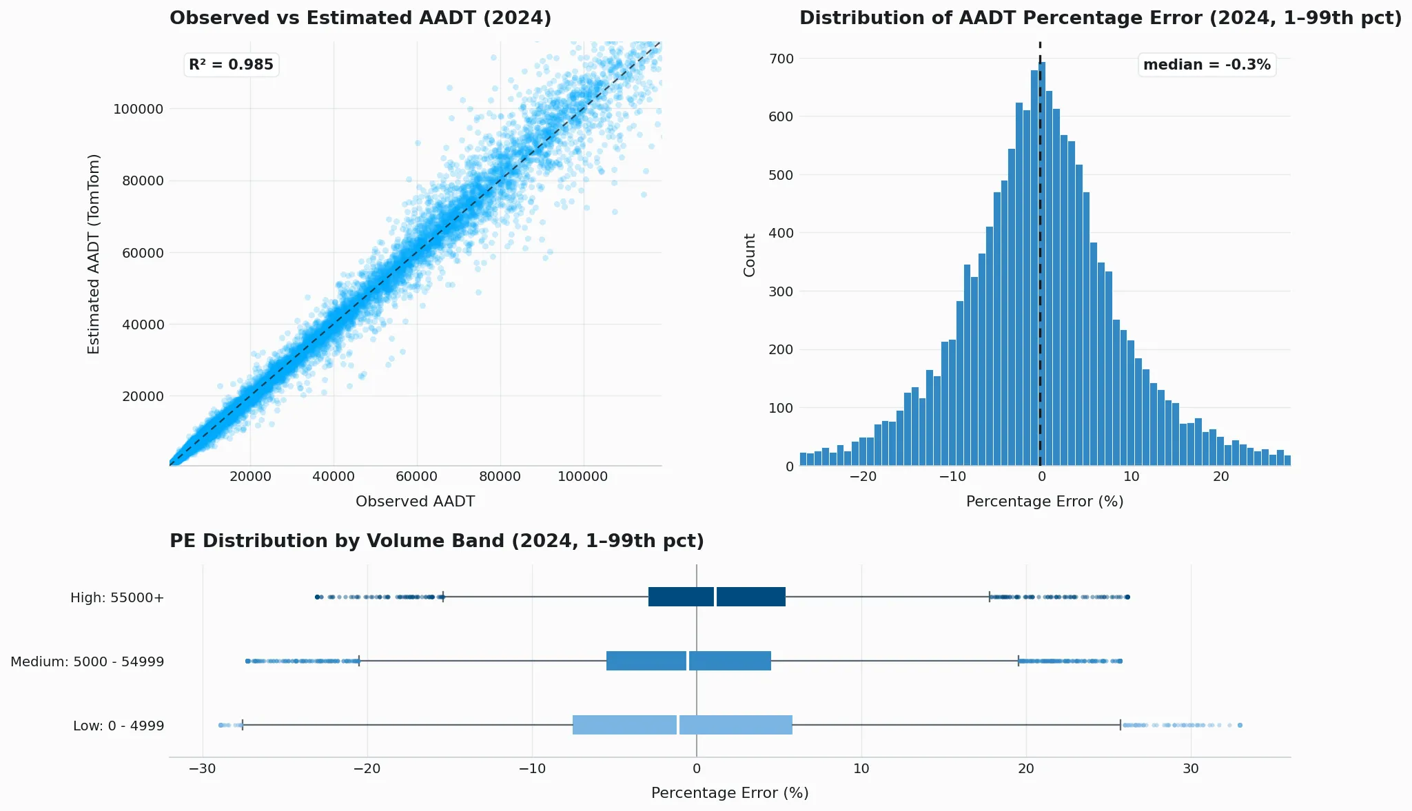
| All roads | 15,518 | 7.6 | 8.5 | 22.6 | -0.2 | 0.85 |
| High (55,000+) | 3,112 | 6.4 | 7.2 | 19.2 | 1.1 | 0.74 |
| Medium (5,000–54,999) | 8,513 | 7.4 | 8.2 | 21.6 | -0.5 | 0.86 |
| Low (under 5,000) | 3,893 | 9.2 | 10.4 | 26.1 | -1.0 | 0.92 |
AAWHT
| Road Category | Counters | MAPE (%) | SQV (15th Pct) |
|---|---|---|---|
| All roads | 14,231 | 9.1 | 0.88 |
| High (55,000+) | 2,898 | 7.1 | 0.80 |
| Medium (5,000–54,999) | 7,766 | 8.8 | 0.88 |
| Low (under 5,000) | 3,567 | 11.6 | 0.93 |
The United States sits mid-pack overall (MAPE 7.6%, SQV 0.85), with healthy low and medium bands (SQV 0.92 and 0.86). The high band is the country’s weak spot, falling to Insufficient at SQV 0.74 and showing a positive median PE (+1.1%) in contrast to the slight negative bias seen elsewhere.
7.8 Unseen countries (LOCO)
AADT
| Road Category | Counters | MAPE (%) | 68th Pct APE (%) | 95th Pct APE (%) | Median PE (%) | SQV (15th Pct) |
|---|---|---|---|---|---|---|
| All roads | 39,187 | 12.9 | 15.7 | 32.8 | -0.5 | 0.76 |
| High (55,000+) | 3,726 | 12.6 | 16.2 | 27.7 | 0.4 | 0.64 |
| Medium (5,000–54,999) | 25,655 | 12.2 | 14.9 | 31.2 | -0.6 | 0.76 |
| Low (under 5,000) | 9,806 | 14.9 | 17.7 | 38.6 | -0.6 | 0.89 |
AAWHT
| Road Category | Counters | MAPE (%) | SQV (15th Pct) |
|---|---|---|---|
| All roads | 68,640 | 18.6 | 0.78 |
| High (55,000+) | 5,992 | 13.9 | 0.69 |
| Medium (5,000–54,999) | 47,226 | 18.4 | 0.77 |
| Low (under 5,000) | 15,422 | 21.4 | 0.87 |
Pooled across the countries withheld from training, the all-roads AADT MAPE of 12.9% sits above that of every country in this assessment (4.8% to 9.7%), the expected cost of predicting without local training data, while the median percentage error of -0.5% shows no systematic bias. The SQV is Acceptable on all roads (0.76) and in the medium band (0.76) and Insufficient in the high band (0.64), whereas the low band stays Good (0.89) despite carrying the highest AADT band MAPE (14.9%), the usual sign of small denominators inflating percentage errors while absolute errors remain controlled.
8. What the results mean for your use case
8.1 For business decision-makers and analysts
Traffic volume data informs strategic decisions (Section 2). For most analytical applications, the question comes down to one thing: is the error range acceptable for the decision at hand?
A practical guide: a MAPE of 10% on a road carrying 20,000 vehicles per day means that estimates differ from the true figure by about 2,000 vehicles on average, and the 68th and 95th percentile columns in Section 7 show how wide the error gets on a single road. For retail site selection, insurance risk modeling or transport infrastructure planning, an error of this size is usually acceptable. For applications that need precise capacity calculations, such as junction design or traffic signal optimization, we recommend adding local count data to the volume estimates where it is available and practicable. For comparisons across time, such as a before-and-after study, Section 9 explains how to read a difference between two periods against the stated accuracy, and how model improvements reach past periods.
Low-volume roads (under 5,000 vehicles per day) tend to show higher MAPE values (Das & Tsapakis, 2020). On roads with very low daily volumes, a higher percentage error still means a small number of vehicles — the worked example in Section 4.1 (a MAPE of 15% on a road carrying 300 vehicles per day, about 45 vehicles) shows the scale. For use cases that depend on individual low-volume rural roads, treat the estimates as indicative and validate them against available count data where precision matters.
8.2 For data scientists and transport modelers
The SQV 15th percentile is a conservative quality indicator (Section 4.4 explains how to read it). When you integrate TomTom Historical Traffic Volumes into a transport model, the SQV shows which road categories you can use with confidence and where extra validation against local counts is advisable.
For road categories with SQV values at or above 0.80 (Fair or better), the data is suitable for transport models and analytical workflows that need segment-level accuracy. For categories between 0.75 and 0.79 (Acceptable), use the data for aggregate and indicative purposes and validate individual segments against local counts. For categories below 0.75 (Insufficient), treat the data as indicative and apply extra quality filters or local calibration where precision is required.
The AAWHT results carry the same guidance for the weekly profile. Where a road category reaches Fair or better on AAWHT, the profile is reliable enough for time-of-day analysis, such as peak-hour shares or the split between weekdays and weekends; where it does not, aggregate the profile to the day before using it. AAWHT describes the typical hour of the week; the accuracy of an estimate for a specific date and hour is documented in the Hourly volumes section.
Where the median percentage error (bias) of a category is close to zero, aggregate measures such as total vehicle kilometers traveled across a network, or the average AADT for a road class, are reliable even where individual segments carry errors. Where a category shows a negative median percentage error (a tendency to under-predict), account for it in applications where absolute volume totals matter.
9. Updates, versions and comparability
9.1 Estimates are updated
TomTom Historical Traffic Volumes is a modeled product. We improve the model continuously, and an improved model can recompute the periods we have already published. A figure for a past period can therefore improve after publication: the recomputed estimate reflects a better model, while the traffic that occurred is unchanged. Regenerating the history in this way keeps a series internally consistent, because every period in it comes from the same model.
9.2 Comparing periods
Every estimate in this product is a measurement with a stated accuracy: the quality figures in Section 7 give it for each country, and pooled for unseen markets, by road category. A comparison between two periods, in a before-and-after study, a year-over-year trend or network monitoring, is a comparison between two such measurements.
AADT and AAWHT aggregate a year of observations, so short-term variation in the probe data largely averages out, and they are the natural basis for year-over-year comparison.
Our guidance: read a difference between two periods against the accuracy figures published for both periods. When we regenerate the history, refresh both periods, so that they come from the same model.
We will extend this guidance as the product evolves.
10. Summary
This document reports the accuracy of the TomTom Historical Traffic Volumes annual averages, AADT and AAWHT, for 2024, measured against independent ground-truth counts in seven countries by k-fold cross-validation, and for markets beyond them by leave-one-country-out (LOCO) validation.
In the 2024 assessment the United Kingdom leads with an all-roads AADT MAPE of 4.8%, and all seven countries keep their all-roads MAPE below 10%, most pairing it with a Good or Very good SQV. Median percentage errors are close to zero throughout, so aggregate network-level measures can be used with confidence. For countries held out from training, the pooled LOCO results give an all-roads AADT MAPE of 12.9% (SQV 0.76), the accuracy to expect where the model has no local training data.
Sweden’s results carry the widest upper error tail of the group (95th percentile APE above 30%) on the smallest national sample (855 counters); readers using segment-level data should consult the band-level tables and the guidance in Section 8.2.
On low-volume roads, MAPE values tend to be higher in percentage terms; as Section 4.1 explains, the difference in vehicles on these roads is typically small.
For markets beyond the seven countries in this k-fold validation, the pooled leave-one-country-out (LOCO) results in Section 7.8 provide the accuracy basis (Section 6).
We publish the results for every validated country, including where they fall short of the quality thresholds in Section 4.4. With this document, customers have what they need to use TomTom Historical Traffic Volumes with a clear view of both its accuracy and its limits.
11. References
Das, S., & Tsapakis, I. (2020). Interpretable machine learning approach in estimating traffic volume on low-volume roadways. International Journal of Transportation Science and Technology, 9(1), 76–88. https://doi.org/10.1016/j.ijtst.2019.09.004
Department for Transport. (2026). TAG Unit M3.1: Highway Assignment Modelling (May 2026). Transport Analysis Guidance. https://www.gov.uk/government/publications/webtag-tag-unit-m3-1-highway-assignment-modelling
Eisinga, K., & Lorkowski, S. (2025). Network-Wide Traffic Volume Estimation Based on Probe Vehicle Data. Transportation Research Record, 2679(4), 264–277. https://doi.org/10.1177/03611981241289408
Federal Highway Administration. (2022). Traffic Monitoring Guide (Version 1.0, December 2022). U.S. Department of Transportation. https://www.fhwa.dot.gov/policyinformation/tmguide/tmg_2022/
Friedrich, M., Pestel, E., Schiller, C., & Simon, R. (2019). Scalable GEH: A Quality Measure for Comparing Observed and Modeled Single Values in a Travel Demand Model Validation. Transportation Research Record, 2673(4), 722–732. https://doi.org/10.1177/0361198119838849
Greenshields, B. D. (1935). A study of traffic capacity. Highway Research Board Proceedings, 14, 448–477. https://onlinepubs.trb.org/Onlinepubs/hrbproceedings/14/14P1-023.pdf
Hastie, T., Tibshirani, R., & Friedman, J. (2009). The Elements of Statistical Learning: Data Mining, Inference, and Prediction (2nd ed.). Springer. https://doi.org/10.1007/978-0-387-84858-7
Herrera, J. C., Work, D. B., Herring, R., Ban, X., Jacobson, Q., & Bayen, A. M. (2010). Evaluation of traffic data obtained via GPS-enabled mobile phones: The Mobile Century field experiment. Transportation Research Part C: Emerging Technologies, 18(4), 568–583. https://doi.org/10.1016/j.trc.2009.10.006
Hyndman, R. J., & Koehler, A. B. (2006). Another look at measures of forecast accuracy. International Journal of Forecasting, 22(4), 679–688. https://doi.org/10.1016/j.ijforecast.2006.03.001
Kerner, B. S. (2004). The Physics of Traffic. Springer. https://doi.org/10.1007/978-3-540-40986-1
Roberts, D. R., Bahn, V., Ciuti, S., Boyce, M. S., Elith, J., Guillera-Arroita, G., Hauenstein, S., Lahoz-Monfort, J. J., Schröder, B., Thuiller, W., Warton, D. I., Wintle, B. A., Hartig, F., & Dormann, C. F. (2017). Cross-validation strategies for data with temporal, spatial, hierarchical, or phylogenetic structure. Ecography, 40(8), 913–929. https://doi.org/10.1111/ecog.02881
Sekuła, P., Marković, N., Vander Laan, Z., & Farokhi Sadabadi, K. (2018). Estimating historical hourly traffic volumes via machine learning and vehicle probe data: A Maryland case study. Transportation Research Part C: Emerging Technologies, 97, 147–158. https://doi.org/10.1016/j.trc.2018.10.012
Transportation Research Board. (2022). Highway Capacity Manual 7th Edition: A Guide for Multimodal Mobility Analysis. National Academies Press. https://doi.org/10.17226/26432
Treiber, M., & Kesting, A. (2013). Traffic Flow Dynamics: Data, Models and Simulation. Springer. https://doi.org/10.1007/978-3-642-32460-4
Zhan, X., Zheng, Y., Yi, X., & Ukkusuri, S. V. (2017). Citywide Traffic Volume Estimation Using Trajectory Data. IEEE Transactions on Knowledge and Data Engineering, 29(2), 272–285. https://doi.org/10.1109/TKDE.2016.2621104